Metal Sphere Radar Cross Section
A 3D simulation demonstrating a the total-field/scattered-field approach on a metallic sphere with a RCS (radar cross section) calculation.
Introduction
This tutorial covers:
The total-field/scattered-field approach
Calculation of a radar cross section (RCS)
Python Script
Get the latest version from git.
Import Libraries
import os, tempfile
from pylab import *

from CSXCAD  import ContinuousStructure
from openEMS import openEMS
from openEMS.physical_constants import *
from openEMS.ports  import UI_data
Setup the simulation
Sim_Path = os.path.join(tempfile.gettempdir(), 'RCS_Sphere')
post_proc_only = False

unit = 1e-3 # all length in mm

sphere_rad = 200

inc_angle = 0 #incident angle (to x-axis) in deg

# size of the simulation box
SimBox = 1200
PW_Box = 750
Setup FDTD parameters & excitation function
FDTD = openEMS(EndCriteria=1e-5)

f_start =  50e6 # start frequency
f_stop  = 1000e6 # stop  frequency
f0      = 500e6
FDTD.SetGaussExcite(  0.5*(f_start+f_stop), 0.5*(f_stop-f_start) )

FDTD.SetBoundaryCond( ['PML_8', 'PML_8', 'PML_8', 'PML_8', 'PML_8', 'PML_8'] )
Setup Geometry & Mesh
CSX = ContinuousStructure()
FDTD.SetCSX(CSX)
mesh = CSX.GetGrid()
mesh.SetDeltaUnit(unit)

#create mesh
mesh.SetLines('x', [-SimBox/2, 0, SimBox/2])
mesh.SmoothMeshLines('x', C0 / f_stop / unit / 20) # cell size: lambda/20
mesh.SetLines('y', mesh.GetLines('x'))
mesh.SetLines('z', mesh.GetLines('x'))
Create a metal sphere and plane wave source
sphere_metal = CSX.AddMetal( 'sphere' ) # create a perfect electric conductor (PEC)
sphere_metal.AddSphere(priority=10, center=[0, 0, 0], radius=sphere_rad)

# plane wave excitation
k_dir = [cos(np.deg2rad(inc_angle)), sin(np.deg2rad(inc_angle)), 0] # plane wave direction
E_dir = [0, 0, 1] # plane wave polarization --> E_z

pw_exc = CSX.AddExcitation('plane_wave', exc_type=10, exc_val=E_dir)
pw_exc.SetPropagationDir(k_dir)
pw_exc.SetFrequency(f0)

start = np.array([-PW_Box/2, -PW_Box/2, -PW_Box/2])
stop  = -start
pw_exc.AddBox(start, stop)

# nf2ff calc
nf2ff = FDTD.CreateNF2FFBox()
Run the simulation
if 0:  # debugging only
    CSX_file = os.path.join(Sim_Path, 'RCS_Sphere.xml')
    if not os.path.exists(Sim_Path):
        os.mkdir(Sim_Path)
    CSX.Write2XML(CSX_file)
    from CSXCAD import AppCSXCAD_BIN
    os.system(AppCSXCAD_BIN + ' "{}"'.format(CSX_file))


if not post_proc_only:
    FDTD.Run(Sim_Path, cleanup=True)
Postprocessing & plotting
# get Gaussian pulse strength at frequency f0
ef = UI_data('et', Sim_Path, freq=f0)

Pin = 0.5*norm(E_dir)**2/Z0 * abs(ef.ui_f_val[0])**2
#
nf2ff_res = nf2ff.CalcNF2FF(Sim_Path, f0, 90, arange(-180, 180.1, 2))
RCS = 4*pi/Pin[0]*nf2ff_res.P_rad[0]

fig = figure()
ax  = fig.add_subplot(111, polar=True)
ax.plot( nf2ff_res.phi, RCS[0], 'k-', linewidth=2 )
ax.grid(True)

# calculate RCS over frequency
freq = linspace(f_start,f_stop,100)
ef = UI_data( 'et', Sim_Path, freq ) # time domain/freq domain voltage
Pin = 0.5*norm(E_dir)**2/Z0 * abs(np.array(ef.ui_f_val[0]))**2

nf2ff_res = nf2ff.CalcNF2FF(Sim_Path, freq, 90, 180+inc_angle, outfile='back_nf2ff.h5')

back_scat = np.array([4*pi/Pin[fn]*nf2ff_res.P_rad[fn][0][0] for fn in range(len(freq))])

figure()
plot(freq/1e6,back_scat, linewidth=2)
grid()
xlabel('frequency (MHz)')
ylabel('RCS ($m^2$)')
title('radar cross section')

figure()
semilogy(sphere_rad*unit/C0*freq,back_scat/(pi*sphere_rad*unit*sphere_rad*unit), linewidth=2)
ylim([10^-2, 10^1])
grid()
xlabel('sphere radius / wavelength')
ylabel('RCS / ($\pi a^2$)')
title('normalized radar cross section')

show()
Images
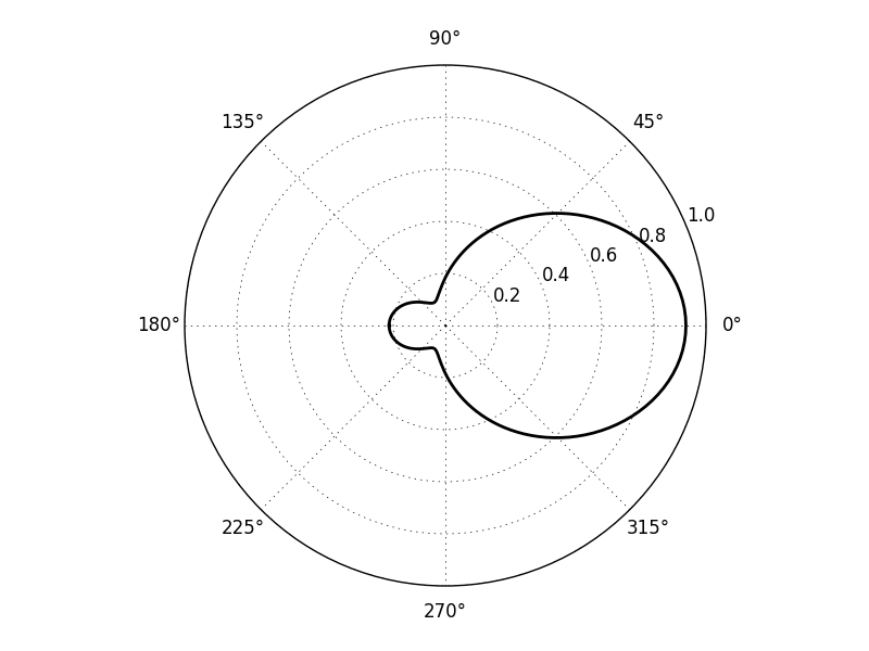
Radar cross section pattern
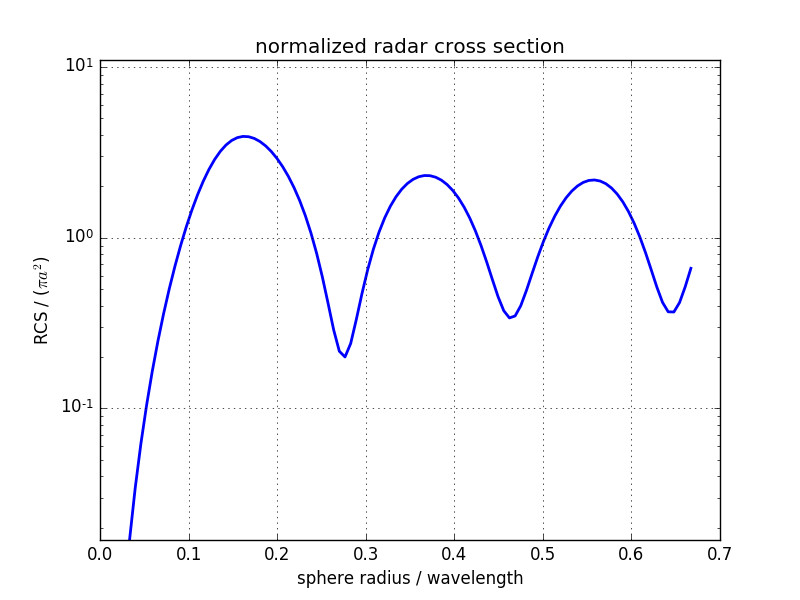
Normalized radar cross Section over normalized wavelength