Rectangular Waveguide
A simple rectangular waveguide, showing the openEMS mode profile capabilities.
Introduction
This tutorial covers:
Setup a mode profile excitation
Create voltage and current probes using the mode profile
Calculate the waveguide impedance and S-Parameter
Python Script
Get the latest version from git.
Import Libraries
import os, tempfile
from pylab import *

from CSXCAD  import ContinuousStructure
from openEMS import openEMS
from openEMS.physical_constants import *
Setup the simulation
Sim_Path = os.path.join(tempfile.gettempdir(), 'Rect_WG')

post_proc_only = False
unit = 1e-6; #drawing unit in um

# waveguide dimensions
# WR42
a = 10700;   #waveguide width
b = 4300;    #waveguide height
length = 50000;

# frequency range of interest
f_start = 20e9;
f_0     = 24e9;
f_stop  = 26e9;
lambda0 = C0/f_0/unit;

#waveguide TE-mode definition
TE_mode = 'TE10';

#targeted mesh resolution
mesh_res = lambda0/30
Setup FDTD parameter & excitation function
FDTD = openEMS(NrTS=1e4);
FDTD.SetGaussExcite(0.5*(f_start+f_stop),0.5*(f_stop-f_start));

# boundary conditions
FDTD.SetBoundaryCond([0, 0, 0, 0, 3, 3]);
Setup geometry & mesh
CSX = ContinuousStructure()
FDTD.SetCSX(CSX)
mesh = CSX.GetGrid()
mesh.SetDeltaUnit(unit)

mesh.AddLine('x', [0, a])
mesh.AddLine('y', [0, b])
mesh.AddLine('z', [0, length])
Apply the waveguide port
ports = []
start=[0, 0, 10*mesh_res];
stop =[a, b, 15*mesh_res];
mesh.AddLine('z', [start[2], stop[2]])
ports.append(FDTD.AddRectWaveGuidePort( 0, start, stop, 'z', a*unit, b*unit, TE_mode, 1))

start=[0, 0, length-10*mesh_res];
stop =[a, b, length-15*mesh_res];
mesh.AddLine('z', [start[2], stop[2]])
ports.append(FDTD.AddRectWaveGuidePort( 1, start, stop, 'z', a*unit, b*unit, TE_mode))

mesh.SmoothMeshLines('all', mesh_res, ratio=1.4)
Define dump box…
Et = CSX.AddDump('Et', file_type=0, sub_sampling=[2,2,2])
start = [0, 0, 0];
stop  = [a, b, length];
Et.AddBox(start, stop);
Run the simulation
if 0:  # debugging only
    CSX_file = os.path.join(Sim_Path, 'rect_wg.xml')
    if not os.path.exists(Sim_Path):
        os.mkdir(Sim_Path)
    CSX.Write2XML(CSX_file)
    from CSXCAD import AppCSXCAD_BIN
    os.system(AppCSXCAD_BIN + ' "{}"'.format(CSX_file))

if not post_proc_only:
    FDTD.Run(Sim_Path, cleanup=True)
Postprocessing & plotting
freq = linspace(f_start,f_stop,201)
for port in ports:
    port.CalcPort(Sim_Path, freq)

s11 = ports[0].uf_ref / ports[0].uf_inc
s21 = ports[1].uf_ref / ports[0].uf_inc
ZL  = ports[0].uf_tot / ports[0].if_tot
ZL_a = ports[0].ZL # analytic waveguide impedance
Plot s-parameter
figure()
plot(freq*1e-6,20*log10(abs(s11)),'k-',linewidth=2, label='$S_{11}$')
grid()
plot(freq*1e-6,20*log10(abs(s21)),'r--',linewidth=2, label='$S_{21}$')
legend();
ylabel('S-Parameter (dB)')
xlabel(r'frequency (MHz) $\rightarrow$')
Compare analytic and numerical wave-impedance
figure()
plot(freq*1e-6,real(ZL), linewidth=2, label='$\Re\{Z_L\}$')
grid()
plot(freq*1e-6,imag(ZL),'r--', linewidth=2, label='$\Im\{Z_L\}$')
plot(freq*1e-6,ZL_a,'g-.',linewidth=2, label='$Z_{L, analytic}$')
ylabel('ZL $(\Omega)$')
xlabel(r'frequency (MHz) $\rightarrow$')
legend()

show()
Images
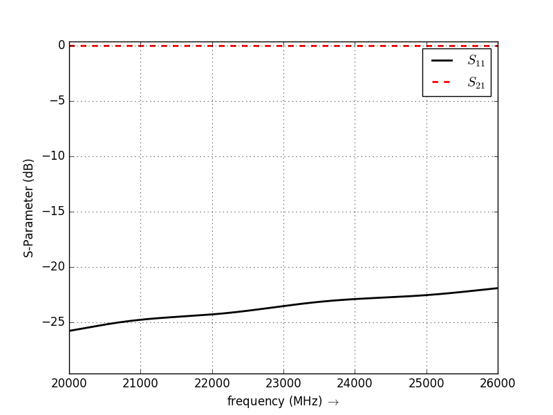
S-Parameter over Frequency